21 - Aspen Plus#
In this exercise we’ll discuss how simulators like Aspen Hysys (Aspen Plus) can be used to estimate unit operation behavior, specifically a flash drum. This is an exercise to give you an introduction to material balances and on vapor liquid equilibrium.
Aspen Plus Software Access#
You’ll log onto one of the CAEDM computers and open Aspen Plus. You can also access that software remotely using ‘labconnect’ for example.
Aspen Help Video#
Link to video that explains a simple flash point calculation or flash drum separation step: Hysys flash drum video
Material Balance Example#
A helpful video of this scenario can be found here: Aspen Plus Flash Drum Example

The conditions in the above equilibrium unit is 50C and 1 bar (see the above video).
#For steady State scenario
Waterin  = 100 # kg/min
Dryairin = 400 # kg/min
VaporOut = 434.936 # kg/min
massFractionwaterVaporout = 1-0.91945 # kg/kg
#First total balance:
LiquidOut = Waterin + Dryairin - VaporOut #This is the liquid out flow rate
#Now the component balance (water):
LiquidOutWater = -massFractionwaterVaporout*VaporOut + Waterin #This is the water balance in the liquid phase flowing out in the LiquidOut stream
print(f'The total liquid flow rate out is {LiquidOut:0.2f} kg/min')
print(f'The amount of water in the liquid phase flowing out is: {LiquidOutWater:0.2f} kg/min')
print (f'The mass fraction of air in the liquid out phase is: {1-LiquidOutWater/LiquidOut:0.5f}')
The total liquid flow rate out is 65.06 kg/min
The amount of water in the liquid phase flowing out is: 64.97 kg/min
The mass fraction of air in the liquid out phase is: 0.00151
#Using Raoult's law:
y_water = (1-0.00446)*0.122/1 #y[i] = x[i]*Psat[i]/P, Psat of water at 50C = 0.122 bar approximately
#mole fraction to mass fraction
ywm = y_water*18/(y_water*18+(1-y_water)*28.97)
1-ywm
0.9208974894233956
Vapor Liquid Equilibrium Background#
The vapor-liquid equilibrium (VLE) of a component or mixture is important in chemical engineering. You’ll take thermodynamics and there spend a significant amount of time on understanding VLE. Simply put, VLE is the ratio of the vapor mole fraction to the liquid mole fraction at a given temperature and pressure.
or for ideal solutions
where \(K\) is the VLE ratio for a given component \(i\), \(y_i\) is the vapor mole fraction, \(x_i\) is the liquid mole fraction, \(P_i^{sat}\) is the saturation pressure of the component, and \(P\) is the total pressure. An ideal solution is one where the vapor and liquid phases are in equilibrium and the saturation pressure is independent of the composition of the liquid phase. Raoult’s law is an example of an ideal solution.
VLE Example Calculation with Python#

The Feed is at the left and the liquid at the bottom and the vapor at the top. The vapor is richer in the more volatile component (methanol) and the liquid is richer in the less volatile component (ethanol).
Given the feed compositions, the total feed, the feed vapor fraction, and the pressure there are five variables to solve for:
The vapor and liquid compositions
The temperature
The vapor and liquid flow rates
The variables are found from solving the following equations assuming an ideal solution for binary system:
# first import packages
import numpy as np
import param
from scipy.optimize import fsolve #import fsolve from scipy.optimize
import scipy.integrate as integrate #import integrate from scipy to get enthalpy
#Define the properties of the components
class component(param.Parameterized):
    Tref = param.Number(298,doc= "K, reference temperature for heat capacity")
    VPcoef = param.List([1,1,1,1,1],doc="Vapor pressure coefficients to yield Psat in Pa, T in K")
    LHCcoef = param.List([1,1,1,1,1],doc="Liquid heat capacity coefficients to yield Cp in J/kmol/K, T in K")
    IGHCcoeff = param.List([1,1,1,1,1],doc="Ideal gas heat capacity coefficients to yield Cp in J/kmol/K, T in K")
    MW = param.Number(1,doc="Molecular weight in kg/kmol")
    Vap = param.Number(1,doc="Heat of Vaporization in J/kmol at 298K(Tref)")

    def Psat(self,T):
        C = self.VPcoef
        return np.exp(C[0]+C[1]/T+ C[2]*np.log(T)+C[3]*T**C[4])
    def Cpig(self,T):
        C = self.IGHCcoeff
        return C[0]+C[1]*(C[2]/T/np.sinh(C[2]/T))**2+C[3]*(C[4]/T/np.cosh(C[4]/T))**2
    def Cpl(self,T):
        C = self.LHCcoef
        return C[0]+C[1]*T+C[2]*T**2+C[3]*T**3+C[4]*T**4
    def Hl(self,T):
        return integrate.quad(self.Cpl,self.Tref,T)[0]
    def Hv(self,T):
        return self.Vap+integrate.quad(self.Cpl,self.Tref,T)[0]

#vapor pressure coefficient estimates
methanol = component(VPcoef=[82.7,-6900,-8.86,7.46E-06,2],\
                LHCcoef=[256000, -2740, 14.8, -0.035, 3.27E-05],\
                    IGHCcoeff=[39250, 87900, 1916, 53650, 896],MW=32.04,Vap=3.75e7)
ethanol = component(VPcoef=[73.3,-7122,-7.14,2.88E-06,2],\
               LHCcoef=[102640,-139.63,-0.030341,0.0020386,0.0],\
                IGHCcoeff=[49200,145770,1660,93900,744],MW=46.07,Vap=4.26e7)
# Define constants
TFlowM = 30 #kg/hr, total flow
VoverL = 0.1 # ratio of the vapor flow rate to the liquid flow rate in the feed
P = 1.6e5 # Pa, pressure of the system
z = np.array([0.95,0.05]) # molar feed composition, methanol, ethanol
#mass fractions
zwm = [z[0]*methanol.MW/(z[0]*methanol.MW+z[1]*ethanol.MW),z[1]*ethanol.MW/(z[0]*methanol.MW+z[1]*ethanol.MW)]
#Total molar flow rate
TFlow = TFlowM*zwm[0]/methanol.MW + TFlowM*zwm[1]/ethanol.MW
#Tref = 298 # K, reference temperature for heat capacity
TFlowM*zwm[0] + TFlowM*zwm[1]
29.999999999999996
# define the function to be solved
def VLE(xvar):
    x = xvar[0] # first element of xvar is the liquid composition of methanol
    y = xvar[1] # next elements of xvar is the vapor composition of methanol
    T = xvar[2] # third element of xvar is the temperature
    L = xvar[3]
    VoverLh = xvar[4]
    V = TFlow*(1 - 1/(1+VoverLh))
    eq = np.zeros(5) # initialize the array of equations
    eq[0] = L*VoverLh + L - TFlow # mass balance
    eq[1] = x*methanol.Psat(T) + (1-x)*ethanol.Psat(T) - P # Raoult's law
    eq[2] = x*L + y*VoverLh*L - TFlow*z[0] # component balance
    eq[3] = (1-x)*ethanol.Psat(T)/P + y - 1 # sum of mole fractions
    #Ethalpy of the Feed
    Vf = TFlow*(1 - 1/(1+VoverL)); Lf = TFlow/(1+VoverL)
    HF = z[0]*(methanol.Hl(T)*Lf+methanol.Hv(T)*Vf)/methanol.MW + z[1]*(ethanol.Hl(T)*Lf+ethanol.Hv(T)*Vf)/ethanol.MW #kJ/hr
    #Ethalpy of the Vapor
    HV = y*methanol.Hv(T)*V/methanol.MW + (1-y)*ethanol.Hv(T)*V/ethanol.MW #kJ/hr
    #Ethanlpy of the Liquid
    HL = x*methanol.Hl(T)*L/methanol.MW + (1-x)*ethanol.Hl(T)*L/ethanol.MW #kJ/hr
    eq[4] = HF - HV - HL
    return eq
# initial guess
xvar0 = np.array([z[0],z[0],350,TFlow/(1+VoverL)*2,VoverL])
VLE(xvar0) # check the function
array([ 9.16268344e-01, -8.17978938e+02,  8.70454927e-01, -1.98048970e-02,
       -1.24141520e+05])
# solve the function
out = fsolve(VLE,xvar0)
Lout = out[3]; Vout = TFlow*(1 - 1/(1+out[4])) #molar basis
Lcomps = [out[0],1-out[0]] #molar compositions
Vcomps = [out[1],1-out[1]] #molar compositions
# on a mass basis:
Lout_M = Lout*Lcomps[0]*methanol.MW + Lout*Lcomps[1]*ethanol.MW
Vout_M = Vout*Vcomps[0]*methanol.MW + Vout*Vcomps[1]*ethanol.MW
print('Check of the mole balance:',TFlow - Lout - Vout) # check the mole balance
print('Check of the mass balance:',TFlowM - Lout_M - Vout_M) # check the mass balance ')
Check of the mole balance: 1.1921019726912618e-13
Check of the mass balance: 3.430771222667772e-10
# print the results
print('The liquid and vapor compositions of methanol are ',out[0:2])
print(f'The temperature is {out[2]-273:.2f} C')
print(f'The liquid and vapor flow rates are {Lout_M:.2f} and {Vout_M:.2f} mol/hr')
print(f'The molar vapor to liquid ratio is {out[4]:.5f}')
The liquid and vapor compositions of methanol are  [0.94815887 0.96849078]
The temperature is 77.16 C
The liquid and vapor flow rates are 27.30 and 2.70 mol/hr
The molar vapor to liquid ratio is 0.09957
#How well did the answer satisfy the equations?
VLE(out)
array([-1.31117339e-13, -3.60887498e-09,  2.40500952e-11,  1.22790667e-13,
        5.90822310e-07])
VLE Example Calculation with Aspen Plus#
Aspen Plus Steps#
Open Aspen Plus
Add a component to the simulation (I added methanol and ethanol)
Specify fluid properties (I used the an Ideal Solution)
Add a separator (Flash2 unit) to the simulation
Specify the inlet and outlet stream names by clicking on the Flowsheet tab and then Global and then the drop down on the Block ID for the unit.
Specify the inlet feed composition, feed vapor fraction, and pressure (the same as specified above for the manual calculation) by then clicking on the streams dropdown tab.
Specify the operating condition of the flash drum by clicking on the Blocks tab and then name of the flash drum and then input. There specify the pressure of the unit and the desired vapor fraction (by mass) of the outlets.
Press the play button to run the simulation
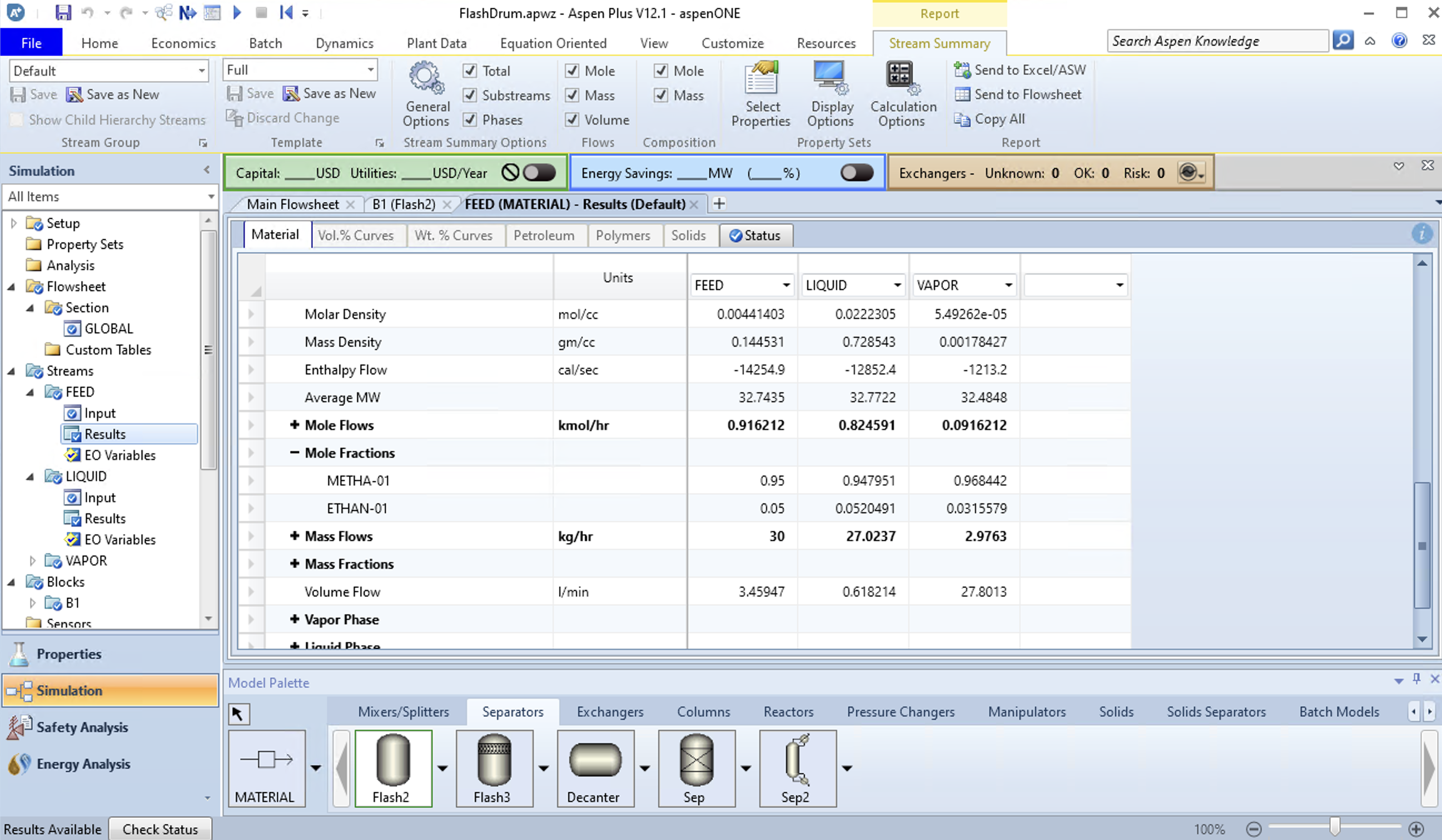
Compared to the above manual results, the ideal solutions agree fairly well despite differences in the vapor pressure and enthalpies. If you specify a different fluid package that includes non-idealities in the solution, you’ll get a slightly different answer (hopefully a more accurate answer).
You should look to do this in your future work as an engineer: Check your answer. Never use just one source. Or in other words, doubt that you got the right answer until you prove to yourself otherwise.
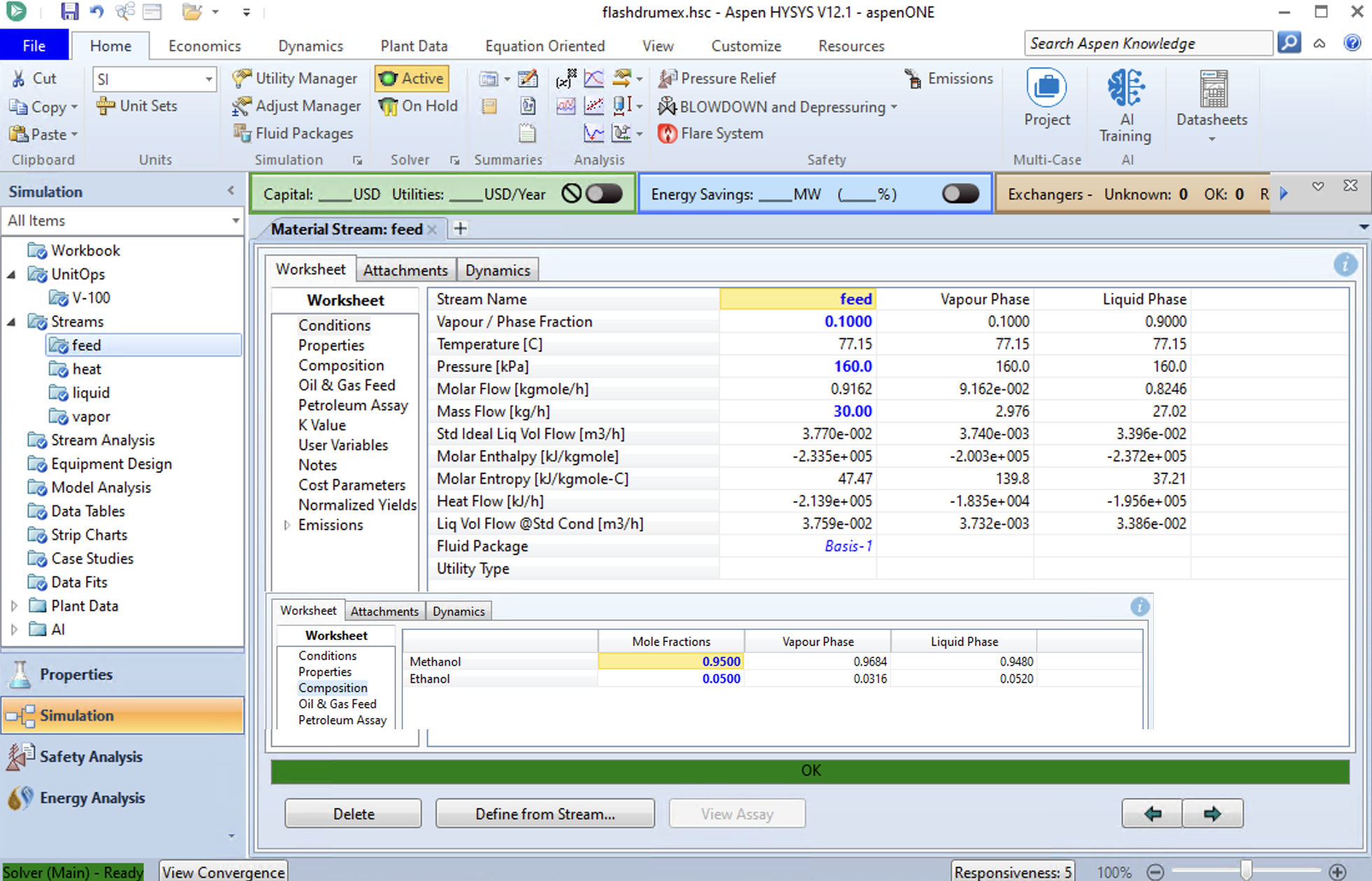
Aspen HySyS Result for a Flash Drum#
The same simulation can be run in Aspen Hysys. The below image shows the results for an Antione Fluid package (ideal solution). The results are similar to Aspen Plus.
Aspen Plus has more compounds.
Additional Simulation Options#
You can add complexity by adding a pressure drop through the flash drum (like when the feed may be forced through an orifice). You can also add a heat source to evaporate more material such that the vapor flow rate is increased.