HW13: Regression and Interpolation#
Regression is an important skill to use data to create a relationship that could be used to describe that data.
Problem 1: Rate Equation and Fitting#
The Arrhenius Equation relates the rate equation of a reaction to the temperature of the reaction. The equation is given by:
where \(k\) is the rate constant, \(A\) is the pre-exponential factor, \(E_a\) is the activation energy, \(R\) is the gas constant, and \(T\) is the temperature in Kelvin.
For a first order reaction, the rate equation is given by:
where \(C_A\) is the concentration of species \(A\).
import numpy as np
import matplotlib.pyplot as plt
#Data from research team
Temp = np.array([100, 110, 120, 130, 140, 150, 160, 170, 180]) # in Celsius
k = np.array([8031385.90210512,  9172549.4982323 , 15836234.10003797, \
       18528434.62455682, 29494725.27289638, 28167947.98802359, \
       33220622.03710192, 49115522.07065894, 51245134.59894557]) #rate constant in 1/s
plt.plot(Temp, k, 'o')
plt.xlabel('Temperature (K)'); plt.ylabel('kA (1/s)')
plt.show()
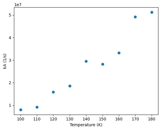
Action, fit the above data to the Arrhenius equation and determine the pre-exponential factor, \(A\) and activation energy, \(Ea\), using the exponential function as written above
Hints:
Use the minimize or curve_fit functions to fit the original data to the Arrhenius equation after defining an Arrhenius function.
Remember to convert the temperature to Kelvin before using it in the equations (Temp given in C. Temp in C + 273.15 = Temp in K).
Action, fit the above data to the Arrhenius equation and determine the pre-exponential factor and activation energy using the linearized version of the equation. Again determine the \(E_a\) and \(A\) values. The linearized version is:
where \(\ln\) is the natural log function. You’ll fit the data by generating new variables where the x is 1/T and the y is ln(k). The slope is then \(-E_a/R\) and the intercept is \(\ln(A)\).
Hints:
Use the polyfit function (order 1) to fit the linearized data to a linear equation.
Remember to convert the temperature to Kelvin before using it in the equations (Temp given in C. Temp in C + 273.15 = Temp in K).
Action, plot the data and the two fits on the same graph. Include a legend and label the axes.
Action Compare your answers by comparing the R2 and MAPE values for both approaches.
Hint:
Make sure to make your comparisons on the original data, not the transformed data.
Problem 2:#
The model for a first-order system with time delay is given by:
where \(y(t)\) is the response, \(t\) is the time, \(\theta\) is the time delay, \(\tau\) is the time constant, and \(S(t)\) is the step function. The step function is defined as:
This system is first-order with a time delay which is common in many chemical engineering systems. You will learn more about this in ChEn 436, Process Control and Dynamics.
Using Pandas, read in the data in the file HW11_P2_Data.csv found here: clint-bg/comptools. The data is y as a function of time.
Action Find the time constant and the time delay for the data. Use the curve_fit function to fit the data to the model.
Action Plot the data and the fit on the same graph. Include a legend and label the axes.
Action Determine the R2 and MAPE values for the fit.
Problem 3:#
Interpolation is used to estimate values between known data points. In this problem, you will use interpolation to estimate the value of a function at a point between two known data points.
The steam tables list the values of multiple properties at various temperatures at intervals of 10C. For example, the below table lists the enthalpy of water at various temperatures (made up data).
Temperature (C) |
Enthalpy (kJ/kg) |
|---|---|
0 |
2500.9 |
10 |
2510.4 |
20 |
2520.0 |
30 |
2529.7 |
40 |
2539.5 |
50 |
2549.4 |
60 |
2559.4 |
70 |
2569.5 |
Action Use interp1D and cubic spline methods to estimate the enthalpy at 25C. The interp1D method was discussed in class. The cubic spline method can be found online here: https://docs.scipy.org/doc/scipy/reference/generated/scipy.interpolate.CubicSpline.html.
Action Compare and comment on the results of the two methods.