Mass (mole) and energy balance problems are fundamental to chemical engineering. It takes practice to understand how to set up and solve these problems. These problems are part of multiple courses in chemical engineering, and they are also part of the Fundamentals of Engineering (FE) exam and proficiency exams given by chemical engineering departments. This course is the 2nd or 3rd time reviewing theses principles. Example exam results demonstrating that more practice is needed are shown below.
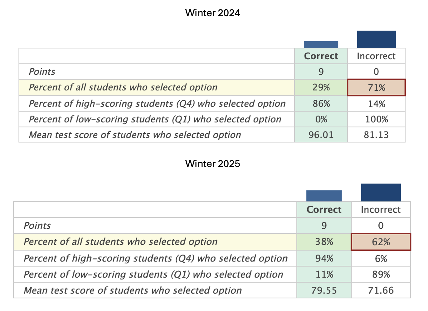
Figure 1:Mass Balance Example Exam Results
Mass and Energy Balances
Helpful sheet: General Mass and Balance Equations
Species Balances
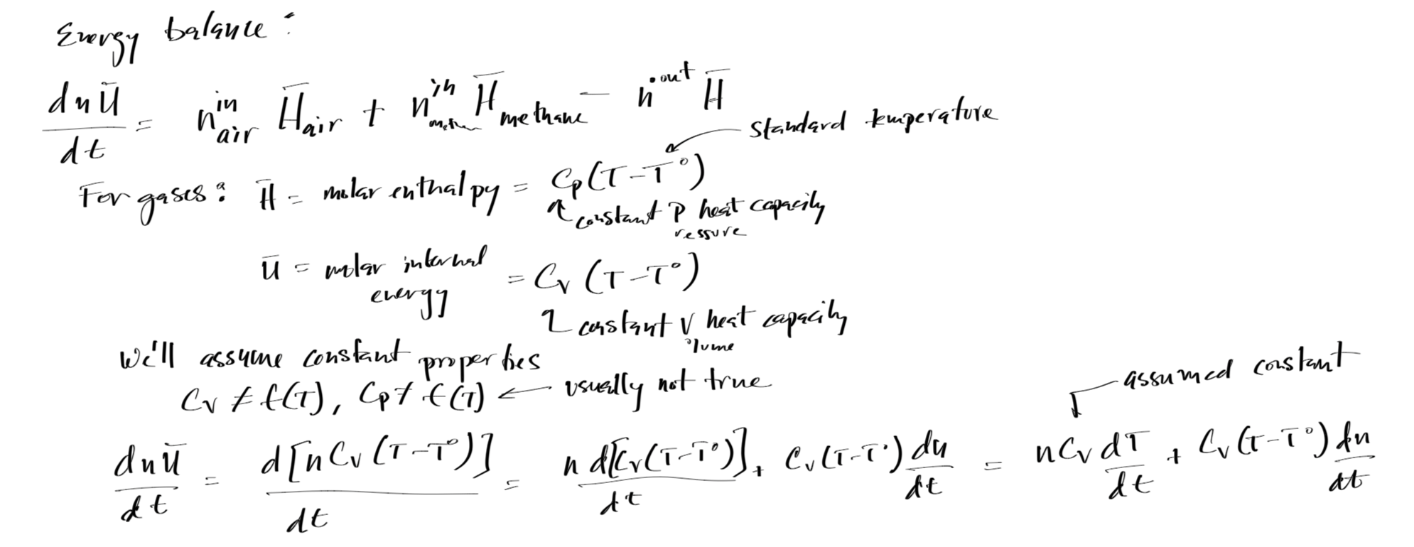
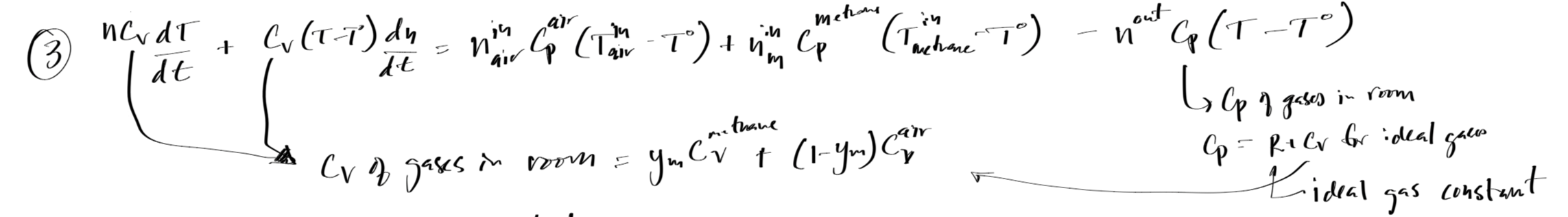
Energy Balance
Why?: Concentration Estimates for Assessing Risk
Prior to implementing control techniques, it can be important to quantify the risk of exposure from a spill scenario of other toxic gas/ vapor release.
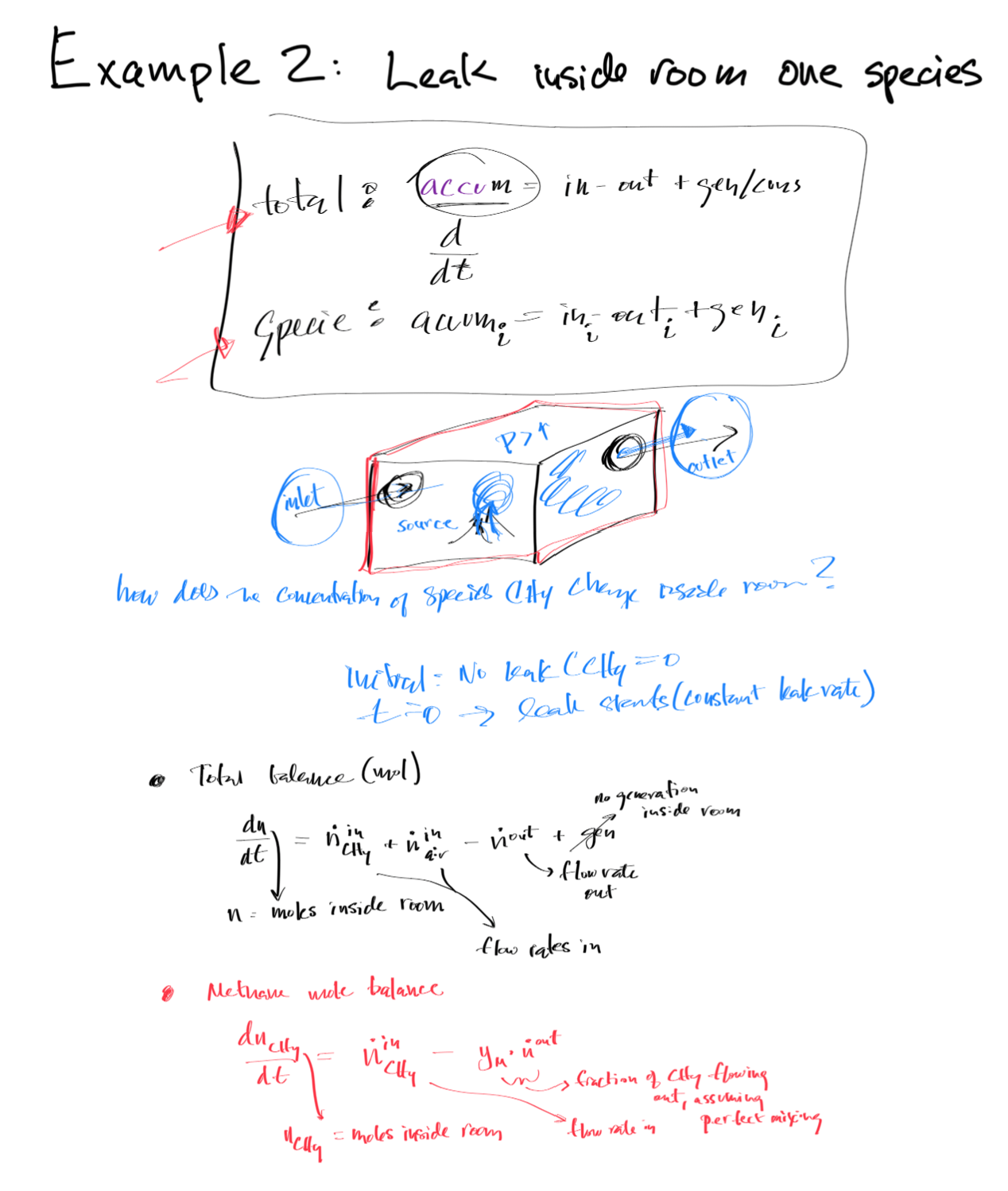
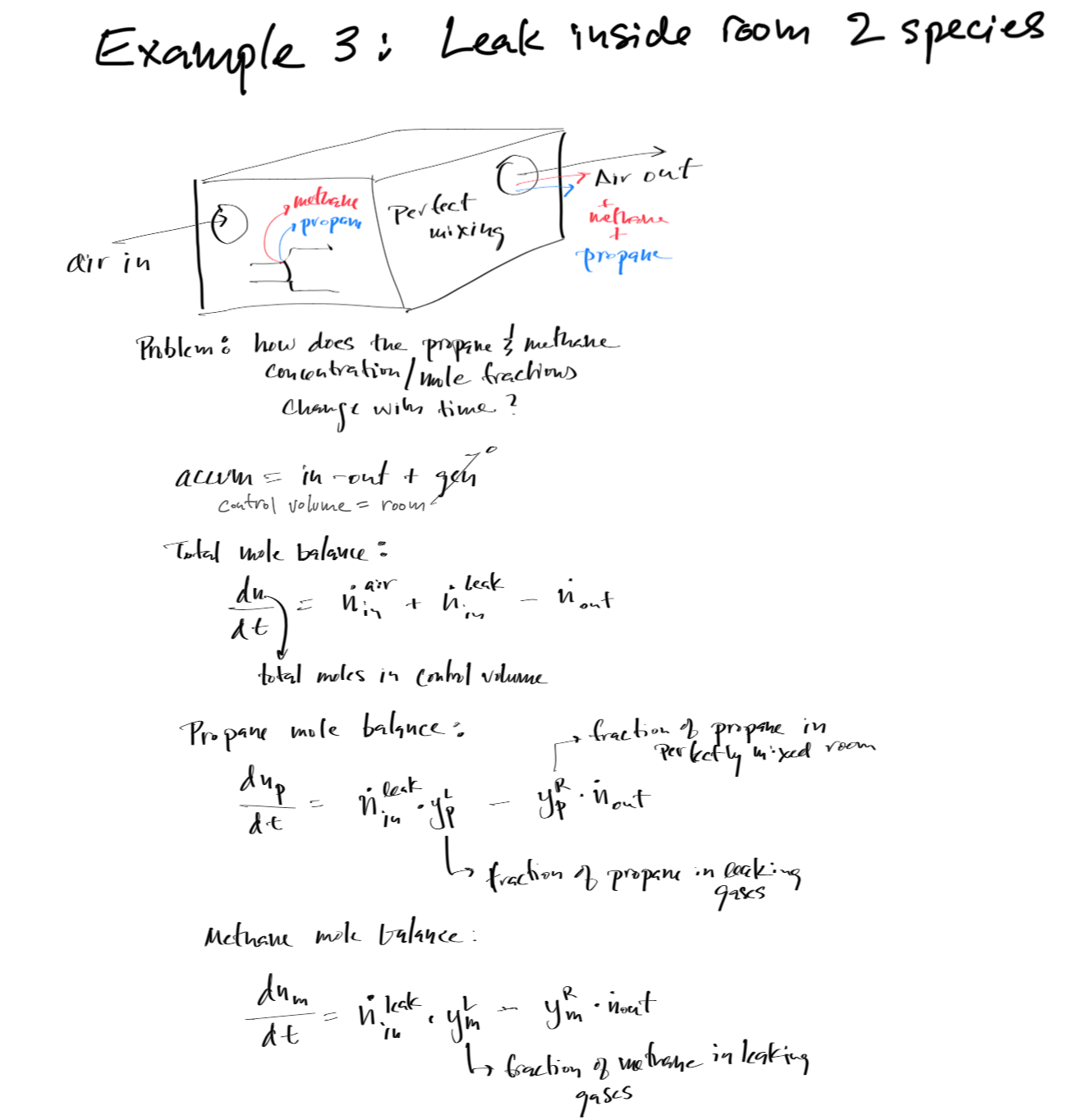
Total Mole (Mass) and Component Mole Balances
Given a control volume and:
A release of toxic gas or vapor at a constant rate
Addition of air at a constant rate
Exit of the gasses based on the inlet conditions and assuming that the exit rate can be achieved without pressurization of the control volume
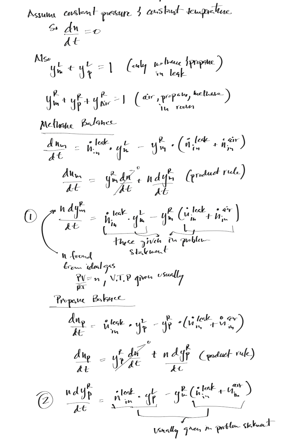
Steady state conditions
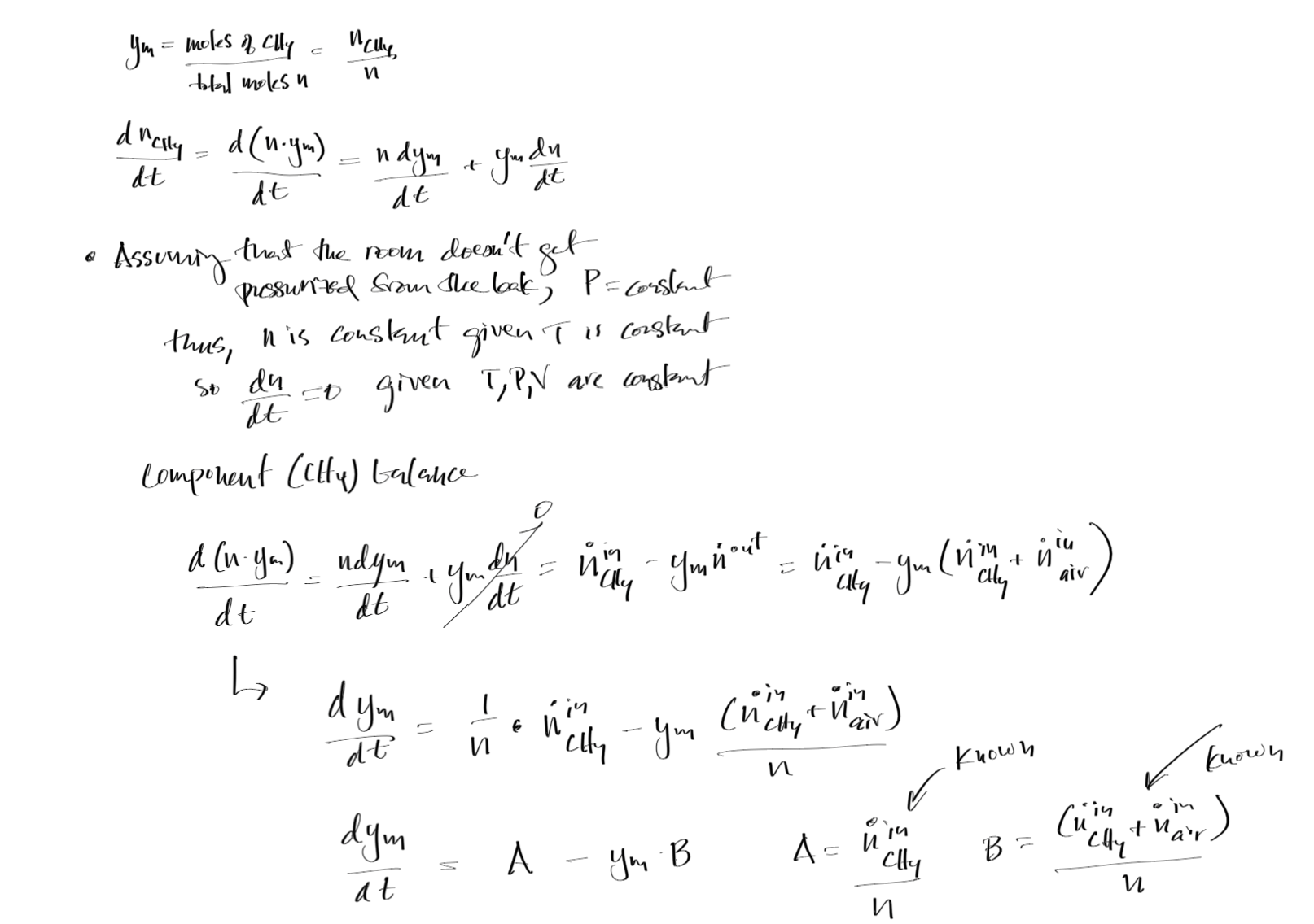
At steady state, the accumulation terms ( and ) are zero.
Other assumptions/ notation:
concentration of interest, ,
the exit rate of the total gases is , mol//time,
the inlet rate of the composition of interest is , mol//time,
, where is the concentration in parts per million (ppm), is the ideal gas constant, is the temperature, and is the pressure.
, for the case of a spill or release of a toxic gas or vapor (new species are not generated).
Perfect mixing of the gases in the control volume (no concentration gradients).
As such, the mole balance for the component of interest i is
If however, there are concentration gradients, the concentration could deviate significantly from the above estimate (larger or smaller).
Inlet composition from vaporization of a liquid
The inlet rate of the species of interest, , can be estimated from the vapor pressure of the liquid and the rate of vaporization and a mass transfer coefficient according to:
where is the mass transfer coefficient, is the saturation concentration of the species close to the liquid surface, and C is the concentration of the species in the air, and is the area of the spill.
can be estimated from correlations or from experimental data or by comparison to another component with a known mass transfer coefficient (e.g. water, ).:
where is the molecular weight of the species of interest and is the molecular weight of water. is typically in the range of depending on the conditions.
can be estimated from the Antoine equation:
where is the saturation pressure of the species of interest, and , , and are constants that can be found in the literature. Where = .
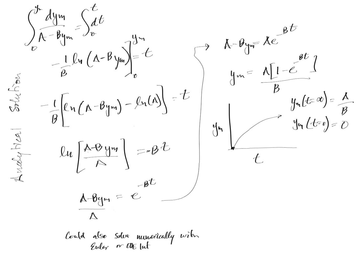
How would you solve the above if you would like the unsteady state concentration as a function of time? And there by obtain the Time Weighted Average (TWA) for a worker directly after a spill?
See here to view a video on a mole (mass) balance for a spill scenario. This video can be helpful for the homework. You can download the sheet used in the video here: supportfiles
Additional Mass Balance Examples
Mass and Energy Balance Example
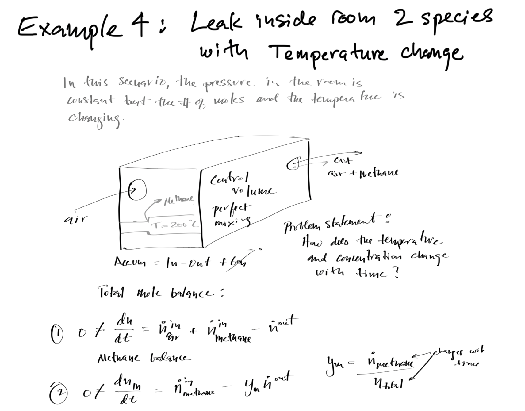
#Mass and energy balance solution for Example 4
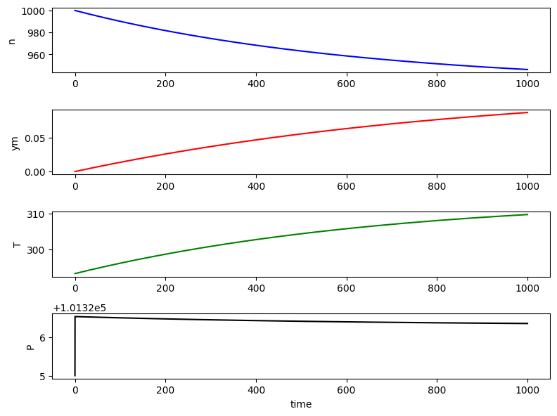
# air flow into room at 20C, methane flow into room at 200C, air/methane mixture leaves the room
# determine the fraction of methane and air temperature as a function of time
import numpy as np
import matplotlib.pyplot as plt
from scipy.integrate import odeint
# Parameters
Cv_m = 27 # J/mol-K specific heat of methane, (estimate) assumed constant but is a function of temperature
Cv_air = 29 # J/mol-K specific heat of air, (estimated) assumed constant but is a function of temperature
#stream flow rates
nin_air = 1 # mol/s air flow rate
nin_m = 1/7 # mol/s methane flow rate
#stream temperatures
Pairin = 101425 # Pa, pressure of air stream entering the room
Tairin = 20 + 273.15 # K, temperature of air entering the room
Tmin = 200 + 273.15 # K, temperature of methane entering the room
#room parameters
orifice_diameter = 0.2 # m (outlet diameter)
Cd = 0.6 # discharge coefficient
Pext = 101325 # Pa, external pressure
P_initial = Pext # Pa, constant pressure
T_initial = 20 + 273.15 # K, initial temperature of room
n_initial = 1000 # total moles in room, can be found from the volume and initial temperature and pressure
nm_initial = 0 # initial moles of methane in room
Rg = 8.314 # J/mol-K
T0 = 20 + 273.15 # K, reference temperature
Pref = 101325 # Pa, constant pressure
Vol = n_initial * Rg* T_initial/P_initial # m^3, volume of room
print(f'Volume of room = {Vol} m^3')
print(f'Air flow rate into room = {nin_air*Rg*Tairin/Pairin} m3/s')
print(f'Air flow rate into room = {nin_air} mol/s')
def derivatives(p,t):
# changing parameters
n, nm, T = p
ym = nm/n
Cv = ym * Cv_m + (1-ym) * Cv_air # J/mol-K, specific heat of the mixture
Mw = ym * 0.016 + (1-ym) * 0.029 # kg/mol, molecular weight of the mixture
P = n*Rg*T/Vol # Pa, pressure in the room
rho = P*Mw/Rg/T # kg/m^3, density of the mixture
# flow rate out, assume flow out is incompressible
nout = Cd * np.pi/4 * orifice_diameter**2 * np.sqrt(2*(P-Pext)*rho)/Mw # mol/s
# Mass balance
# first total mass balance
dndt = nin_air + nin_m - nout
# then component balance
dnmdt = nin_m - nout * ym
# Energy balance
dTdt = 1/(n*Cv)*(- Cv*(T-T0)*dndt + nin_air*(Cv_air+Rg)*(Tairin-T0) + nin_m*(Cv_m+Rg)*(Tmin-T0) - nout*(Cv+Rg)*(T-T0))
return [dndt, dnmdt, dTdt]
# time points
t = np.linspace(0,1000,10000) # seconds
# solve ODE
n0 = [n_initial, nm_initial, T_initial]
sol = odeint(derivatives, n0, t)
# plot results in a grid of subplots
fig, ax = plt.subplots(4, 1, figsize=(8, 6))
ax[0].plot(t, sol[:, 0], 'b', label='n')
ax[0].set_ylabel('n')
ax[1].plot(t, sol[:, 1]/sol[:,0], 'r', label='ym')
ax[1].set_ylabel('ym')
ax[2].plot(t, sol[:, 2], 'g', label='T')
ax[2].set_ylabel('T')
ax[3].plot(t, sol[:, 0]*Rg*sol[:,2]/Vol, 'k', label='P')
ax[3].set_ylabel('P')
ax[3].set_xlabel('time')
fig.tight_layout(pad = 1.0)
plt.show()
Volume of room = 24.053778435726617 m^3
Air flow rate into room = 0.024030062607838305 m3/s
Air flow rate into room = 1 mol/s
- Guymon, C. (2025). Foundations of Spiritual and Physical Safety: with Chemical Processes.